Procedures as General Methods

We introduced compound procedures in section  as a mechanism for abstracting patterns of numerical operations so as to make them independent of the particular numbers involved. With higher-order procedures, such as the integral procedure of section , we began to see a more powerful kind of abstraction: procedures used to express general methods of computation, independent of the particular functions involved. In this section we discuss two more elaborate examples--general methods for finding zeros and fixed points of functions--and show how these methods can be expressed directly as procedures.

Finding roots of equations by the half-interval method

The half-interval method is a simple but powerful technique for finding roots of an equation f(x)=0, where f is a continuous function. The idea is that, if we are given points a and b such that f(a) < 0 < f(b), then f must have at least one zero between a and b. To locate a zero, let x be the average of a and b and compute f(x). If f(x) > 0, then f must have a zero between a and x. If f(x) < 0, then f must have a zero between x and b. Continuing in this way, we can identify smaller and smaller intervals on which f must have a zero. When we reach a point where the interval is small enough, the process stops. Since the interval of uncertainty is reduced by half at each step of the process, the number of steps required grows as , where L is the length of the original interval and T is the error tolerance (that is, the size of the interval we will consider ``small enough''). Here is a procedure that implements this strategy:

(define (search f neg-point pos-point)
  (let ((midpoint (average neg-point pos-point)))
    (if (close-enough? neg-point pos-point)
        midpoint
        (let ((test-value (f midpoint)))
          (cond ((positive? test-value)
                 (search f neg-point midpoint))
                ((negative? test-value)
                 (search f midpoint pos-point))
                (else midpoint))))))

We assume that we are initially given the function f together with points at which its values are negative and positive. We first compute the midpoint of the two given points. Next we check to see if the given interval is small enough, and if so we simply return the midpoint as our answer. Otherwise, we compute as a test value the value of f at the midpoint. If the test value is positive, then we continue the process with a new interval running from the original negative point to the midpoint. If the test value is negative, we continue with the interval from the midpoint to the positive point. Finally, there is the possibility that the test value is 0, in which case the midpoint is itself the root we are searching for.

To test whether the endpoints are ``close enough'' we can use a procedure similar to the one used in section  for computing square roots:

(define (close-enough? x y)
  (< (abs (- x y)) 0.001))

Search is awkward to use directly, because we can accidentally give it points at which f's values do not have the required sign, in which case we get a wrong answer. Instead we will use search via the following procedure, which checks to see which of the endpoints has a negative function value and which has a positive value, and calls the search procedure accordingly. If the function has the same sign on the two given points, the half-interval method cannot be used, in which case the procedure signals an error.

(define (half-interval-method f a b)
  (let ((a-value (f a))
        (b-value (f b)))
    (cond ((and (negative? a-value) (positive? b-value))
           (search f a b))
          ((and (negative? b-value) (positive? a-value))
           (search f b a))
          (else
           (error "Values are not of opposite sign" a b)))))

The following example uses the half-interval method to approximate as the root between 2 and 4 of :

(half-interval-method sin 2.0 4.0)
3.14111328125

Here is another example, using the half-interval method to search for a root of the equation x³ - 2x - 3 = 0 between 1 and 2:

(half-interval-method (lambda (x) (- (* x x x) (* 2 x) 3))
                      1.0
                      2.0)
1.89306640625

Finding fixed points of functions

A number x is called a fixed point of a function f if x satisfies the equation f(x)=x. For some functions f we can locate a fixed point by beginning with an initial guess and applying f repeatedly,

until the value does not change very much. Using this idea, we can devise a procedure fixed-point that takes as inputs a function and an initial guess and produces an approximation to a fixed point of the function. We apply the function repeatedly until we find two successive values whose difference is less than some prescribed tolerance:

(define tolerance 0.00001)

(define (fixed-point f first-guess)
  (define (close-enough? v1 v2)
    (< (abs (- v1 v2)) tolerance))
  (define (try guess)
    (let ((next (f guess)))
      (if (close-enough? guess next)
          next
          (try next))))
  (try first-guess))

For example, we can use this method to approximate the fixed point of the cosine function, starting with 1 as an initial approximation:

(fixed-point cos 1.0)
.7390822985224023

Similarly, we can find a solution to the equation :

(fixed-point (lambda (y) (+ (sin y) (cos y)))
             1.0)
1.2587315962971173

The fixed-point process is reminiscent of the process we used for finding square roots in section . Both are based on the idea of repeatedly improving a guess until the result satisfies some criterion. In fact, we can readily formulate the square-root computation as a fixed-point search. Computing the square root of some number x requires finding a y such that y² = x. Putting this equation into the equivalent form y = x/y, we recognize that we are looking for a fixed point of the function , and we can therefore try to compute square roots as

(define (sqrt x)
  (fixed-point (lambda (y) (/ x y))
               1.0))

Unfortunately, this fixed-point search does not converge. Consider an initial guess y₁. The next guess is y₂ = x/y₁ and the next guess is y₃ = x/y₂ = x/(x/y₁) = y₁. This results in an infinite loop in which the two guesses y₁ and y₂ repeat over and over, oscillating about the answer.

One way to control such oscillations is to prevent the guesses from changing so much. Since the answer is always between our guess y and x/y, we can make a new guess that is not as far from y as x/y by averaging y with x/y, so that the next guess after y is instead of x/y. The process of making such a sequence of guesses is simply the process of looking for a fixed point of :

(define (sqrt x)
  (fixed-point (lambda (y) (average y (/ x y)))
               1.0))

(Note that is a simple transformation of the equation y=x/y; to derive it, add y to both sides of the equation and divide by 2.)

With this modification, the square-root procedure works. In fact, if we unravel the definitions, we can see that the sequence of approximations to the square root generated here is precisely the same as the one generated by our original square-root procedure of section . This approach of averaging successive approximations to a solution, a technique we that we call average damping, often aids the convergence of fixed-point searches.

Exercise. Show that the golden ratio (section ) is a fixed point of the transformation , and use this fact to compute by means of the fixed-point procedure.

Exercise. Modify fixed-point so that it prints the sequence of approximations it generates, using the newline and display primitives shown in exercise . Then find a solution to x^x = 1000 by finding a fixed point of . (Use Scheme's primitive log procedure, which computes natural logarithms.) Compare the number of steps this takes with and without average damping. (Note that you cannot start fixed-point with a guess of 1, as this would cause division by .)  

Exercise. a. An infinite continued fraction is an expression of the form

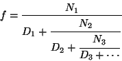
As an example, one can show that the infinite continued fraction expansion with the N_i and the D_i all equal to 1 produces , where is the golden ratio (described in section ). One way to approximate an infinite continued fraction is to truncate the expansion after a given number of terms. Such a truncation--a so-called k-term finite continued fraction--has the form

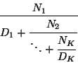
Suppose that n and d are procedures of one argument (the term index i) that return the N_i and D_i of the terms of the continued fraction. Define a procedure cont-frac such that evaluating (cont-frac n d k) computes the value of the k-term finite continued fraction. Check your procedure by approximating using

(cont-frac (lambda (i) 1.0)
           (lambda (i) 1.0)
           k)

for successive values of k. How large must you make k in order to get an approximation that is accurate to 4 decimal places?

b. If your cont-frac procedure generates a recursive process, write one that generates an iterative process. If it generates an iterative process, write one that generates a recursive process.  

Exercise. In 1737, the Swiss mathematician Leonhard Euler published a memoir De Fractionibus Continuis, which included a continued fraction expansion for e-2, where e is the base of the natural logarithms. In this fraction, the N_i are all 1, and the D_i are successively 1, 2, 1, 1, 4, 1, 1, 6, 1, 1, 8, .... Write a program that uses your cont-frac procedure from exercise  to approximate e, based on Euler's expansion.

Exercise. A continued fraction representation of the tangent function was published in 1770 by the German mathematician J.H. Lambert:

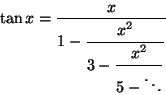
where x is in radians. Define a procedure (tan-cf x k) that computes an approximation to the tangent function based on Lambert's formula. K specifies the number of terms to compute, as in exercise .